Understanding erasure coding
Over time, I went down the rabbit hole of reading about erasure coding on cloud platforms. It’s quite interesting how these players promise 99.999999999% (that’s eleven 9s) of durability for the stored data.
While Backblaze documents this to great detail on their 17+3 (or 15+5) storage design, AWS S3 so far has been a mystery. They provide extensive documentation on their user-facing APIs and interfaces, but offer little insight into the limitations behind their design choices. Their presentation at AWS re:Invent 2024 talks about some of it in detail. Must say that their re:Invent is way more interesting than their documentation. 😀
Erasure coding
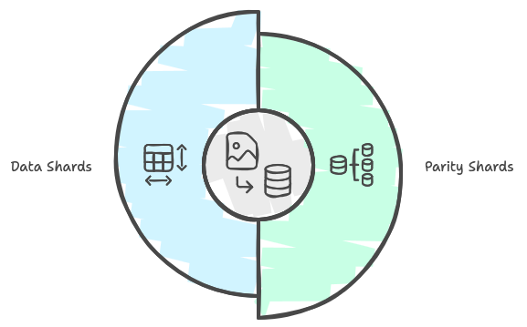
The basic idea behind erasure coding is that drives can fail at any time, and hence, redundancy is needed. One way to have redundancy is to have an exact copy on another disk.
Imagine disk01 and disk02 - both holding the exact same set of bits. Now, if disk01 fails, disk02 will be the only one holding the data. Single disk failures are quite common at scale, and it’s too risky to be holding critical data on disk02 alone for now and that too when it has to be completely read to rebuild the copy. This brings the idea to three copies - store data in disk01, disk02 and disk03.
This works in theory, but has two major challenges:
- If two disks go down, data will be at major risk
- Storage cost has gone 3x.
To address the first challenge, one can add another disk, and now we have disk01, disk02, disk03 and disk04 - each holding the exact same data, and one can lose up to three of them, which is quite reasonable, but this worsens the other issue as now to store x, we are using 4x capacity. To solve this, most storage systems at scale use erasure coding. The idea is to break data into chunks & pass through a pre-defined algorithm and mathematically calculate parity data (often called shards).
In the case of Backblaze design, they break files into 17 pieces (17 data shards) and calculate 3 parity bits (3 data shards). Each of these shards (whether data or parity) is of the same size as the others, and any 17 of these in any mix can reproduce the original data. Thus, storing 20 (17+3) shards across 20 different disks gives the ability to lose up to three drives without losing data. This provides the same fault tolerance as storing 4 identical copies, but instead of 4x storage, it’s just 1.18x storage, which is the real magic. Thus, for around 17.65% overhead on storage, this gives the ability to lose up to three drives without losing data.
In case of AWS S3 (as given in the presentation), they do a 5+4 design (5 data shards, 4 parity shards), giving them 9 shards. They likely went for this because of a number of factors, with one being a number which can be evenly divided by 3. That way, they can store 3+3+3 shards across three different data centres and need only any 5 shards to rebuild the original data.
Tradeoff between shard count and storage overhead
This 5+4 = 9 shards may make one wonder - why not 5+1 = 6 and store 2 + 2 + 2 in each failure zone and store 6 in each zone. Each design: More shards vs Fewer shards — has its own advantages.
Let’s compare a 5+4 Vs 5+1. The number of shards needed to recover data in 5+4 is 5, while in 5+1 it is also 5. This means if all shards are spread around different hard disks, one can lose 4 HDDs in a 5+4 design but only 1 in a 5+1 design. More than 1 HDD loss will cause data loss. Thus, the number of shards fewer than 3 - 4 can be hard (as that’s what defines acceptable HDD failure).
What about high shard count? Why not 11+7 = 18 shards, with 6 going to each failure zone? In case of 11+7, they can lose up to 7 disks with no data loss; however, it will take much more CPU. Also, spreading data to more disks will risk overloading I/O across many disks without much return. Another factor is storage overhead.
Here’s a table to calculate overhead in these configs:
| Scheme | Data Shards | Parity Shards | Disk Failure Tolerance | Storage Overhead |
|---|---|---|---|---|
| 17+3 | 17 | 3 | 3 | 17.65% (3/17) |
| 15+5 | 15 | 5 | 5 | 33.33% (5/15) |
| 5+4 | 5 | 4 | 4 | 80% (4/5) |
| 11+7 | 11 | 7 | 7 | 63.64% (7/11) |
| 11+10 | 11 | 10 | 10 | 90.91% (10/11) |
Backblaze once in their post in 2024 mentioned:
The ratios of data shards to parity shards we currently use are 17/3, 16/4, and 15/5, depending primarily on the size of the drives being used to store the data—the larger the drive, the higher the parity.
This had to do with restore times. For higher capacity drives (16TB), restore time is much higher than a 4TB drive. Thus, when a drive fails in a 17+3 design, they are effectively on 17+2 for a few days. Doing a 15+5 allows them to have tolerance up to 5 disk failures, but for 33.3% overhead (instead of 17.6%).
Playing with erasure coding
Most of these systems are built on Reed-Solomon codes. There are many open source implementations available for it, including from Backblaze - JavaReedSolomon, Go implementation and Python library - pyeclib.
Product-wise, these concepts are available in open source Minio if one is planning to self-host with erasure coding.
I picked up pyeclib and tried with tools from openstack, which provide scripts for simple encode/decode etc.
> python3 pyeclib_encode.py --help
usage: pyeclib_encode.py [-h] k m ec_type file_dir filename fragment_dir

Encoder for PyECLib.

positional arguments:
  k             number of data elements
  m             number of parity elements
  ec_type       EC algorithm used
  file_dir      directory with the file
  filename      file to encode
  fragment_dir  directory to drop encoded fragments

options:
  -h, --help    show this help message and exit
Let’s generate a dummy 1GB file, calculate its checksum, break it into 17+3, restore and do checksum again.
Create a test file
> dd if=/dev/zero of=output_1GB_file.bin bs=1G count=1
1+0 records in
1+0 records out
1073741824 bytes (1.1 GB, 1.0 GiB) copied, 1.1953 s, 898 MB/s

> sha256sum output_1GB_file.bin
49bc20df15e412a64472421e13fe86ff1c5165e18b2afccf160d4dc19fe68a14  output_1GB_file.bin
Now let’s create shards for it based on liberasurecode:
> mkdir shards_17_3

> python3 pyeclib_encode.py 17 3 liberasurecode_rs_vand . output_1GB_file.bin shards_17_3
k = 17, m = 3
ec_type = liberasurecode_rs_vand
filename = output_1GB_file.bin

> ls shards_17_3
output_1GB_file.bin.0   output_1GB_file.bin.11  output_1GB_file.bin.14  output_1GB_file.bin.17  output_1GB_file.bin.2  output_1GB_file.bin.5  output_1GB_file.bin.8
output_1GB_file.bin.1   output_1GB_file.bin.12  output_1GB_file.bin.15  output_1GB_file.bin.18  output_1GB_file.bin.3  output_1GB_file.bin.6  output_1GB_file.bin.9
output_1GB_file.bin.10  output_1GB_file.bin.13  output_1GB_file.bin.16  output_1GB_file.bin.19  output_1GB_file.bin.4  output_1GB_file.bin.7

> du -s output_1GB_file.bin
1048580	output_1GB_file.bin

> du -s shards_17_3
1233684	shards_17_3
Thus, size went up by 185104 bytes (17.65% overhead).
Let’s randomly delete three shards and recover data:
> rm shards_17_3/output_1GB_file.bin.0
> rm shards_17_3/output_1GB_file.bin.10
> rm shards_17_3/output_1GB_file.bin.19

> python3 pyeclib_decode.py 17 3 liberasurecode_rs_vand shards_17_3/output_1GB_file.bin.1 shards_17_3/output_1GB_file.bin.2 shards_17_3/output_1GB_file.bin.3 shards_17_3/output_1GB_file.bin.4 shards_17_3/output_1GB_file.bin.5 shards_17_3/output_1GB_file.bin.6 shards_17_3/output_1GB_file.bin.7 shards_17_3/output_1GB_file.bin.8 shards_17_3/output_1GB_file.bin.9 shards_17_3/output_1GB_file.bin.11 shards_17_3/output_1GB_file.bin.12 shards_17_3/output_1GB_file.bin.13 shards_17_3/output_1GB_file.bin.14 shards_17_3/output_1GB_file.bin.15 shards_17_3/output_1GB_file.bin.16 shards_17_3/output_1GB_file.bin.17 shards_17_3/output_1GB_file.bin.18 recovered-output_1GB_file.bin
k = 17, m = 3
ec_type = liberasurecode_rs_vand
fragments = ['shards_17_3/output_1GB_file.bin.1', 'shards_17_3/output_1GB_file.bin.2', 'shards_17_3/output_1GB_file.bin.3', 'shards_17_3/output_1GB_file.bin.4', 'shards_17_3/output_1GB_file.bin.5', 'shards_17_3/output_1GB_file.bin.6', 'shards_17_3/output_1GB_file.bin.7', 'shards_17_3/output_1GB_file.bin.8', 'shards_17_3/output_1GB_file.bin.9', 'shards_17_3/output_1GB_file.bin.11', 'shards_17_3/output_1GB_file.bin.12', 'shards_17_3/output_1GB_file.bin.13', 'shards_17_3/output_1GB_file.bin.14', 'shards_17_3/output_1GB_file.bin.15', 'shards_17_3/output_1GB_file.bin.16', 'shards_17_3/output_1GB_file.bin.17', 'shards_17_3/output_1GB_file.bin.18']
filename = recovered-output_1GB_file.bin

> sha256sum recovered-output_1GB_file.bin.decoded
49bc20df15e412a64472421e13fe86ff1c5165e18b2afccf160d4dc19fe68a14  recovered-output_1GB_file.bin.decoded
And here’s one similar to what AWS S3 uses:
> mkdir shards_5_4

> python3 pyeclib_encode.py 5 4 liberasurecode_rs_vand . output_1GB_file.bin shards_5_4/
k = 5, m = 4
ec_type = liberasurecode_rs_vand
filename = output_1GB_file.bin

> du -s shards_5_4/
1887448	shards_5_4/
1887448 bytes (80% overhead), which may seem high, but once we consider it’s better than 4x storage and with distribution of 3+3+3 shards in each failure zone, AWS can bear the loss of a full zone and even an additional loss of one shard in the remaining DC and still recover the data.
Storage is fascinating. 😀